
Generalized Skew Laplace Random Fields: Bayesian Spatial Prediction for Skew and Heavy Tailed Data
- DOI
- 10.2991/jsta.d.210111.001How to use a DOI?
- Keywords
- Bayesian spatial prediction; Multivariate generalized skew Laplace distribution; Metropolis–Hastings; Gibbs sampling
- Abstract
Earlier works on spatial prediction issue often assume that the spatial data are realization of Gaussian random field. However, this assumption is not applicable to the skewed and kurtosis distributed data. The closed skew normal distribution has been used in these circumstances. As another alternative, we apply generalized skew Laplace distributions for defining a skew and heavy tailed random field for Bayesian prediction. Simulation study and a real problem are then applied to evaluate the performance of this model.
- Copyright
- © 2021 The Authors. Published by Atlantis Press B.V.
- Open Access
- This is an open access article distributed under the CC BY-NC 4.0 license (http://creativecommons.org/licenses/by-nc/4.0/).
1. INTRODUCTION
Spatial prediction is an important subject in statistical analysis of environmental data which are often spatially correlated. In such cases it is supposed that data come from a Gaussian random field (RF). When spatial data are non-Gaussian but a Gaussian transformation for them exist, Oliveira et al. [1], Oliveira and Ecker [2], Oliveira [3] propose spatial prediction for transformed RFs. However, normalizing transformation is unknown in application and interpretation of the transformed data is also more difficult than original data [4,5]. When distribution of data has an appropriate number of similarities with normal distribution but is asymmetric, Kim and Mallick [6] used a skew Gaussian (SG) RF. Hosseini et al. [7,8] made inference on spatial generalized linear mixed models (SGLMMs) with SG latent variables. Because of some shortage in SG distribution such as nonclosing under conditioning, Dominguez-Molina et al. [9] defined multivariate closed skew normal (CSN) distribution. Karimi and Mohammadzadeh [10,11] and Karimi et al. [12] used CSN RF for Bayesian spatial prediction, Bayesian spatial regression and inversion of seismic data. Hosseini and Mohammadzadeh [13] have done Bayesian prediction for SGLMM with CSG latent variables. However, CSN random variables are not appropriate for modeling data with heavy tails. Since t-distribution is an applicable distribution to real data with heavy tails, Røislien and Omre [14] defined a t-distributed RF, but this RF could not be suitable for modeling the skew data. An appropriate choice for modeling skew and heavy tailed data which is well defined for RF and has some similar characteristics with Gaussian field is multivariate generalized asymmetric Laplace (GAL) distribution introduced by Kozubowski et al. [15]. In this paper, we have applied multivariate GAL distributions for defining the skew and heavy tail RFs. The Bayesian predictions are then achieved by using this RF. A simulation study is performed to check the validity of the model and the proposed prediction method is used on an environmental data set.
A review on the multivariate GAL distribution is presented in Section 2. As in Section 3, the GAL RF is defined, the Bayesian spatial prediction has been considered by GAL RF in Section 4. A simulation study is discussed in Section 5 followed by application of the GAL RF to environmental real data in Section 6.
2. MULTIVARIATE GAL RANDOM VARIABLE
In this section, we review the definition and basic setup of the multivariate GAL distribution introduced by [15].
Definition 2.1
Multivariate GAL law. A continuous p-dimensional random vector
If matrix
We have the following representation for multivariate GAL random variable
If
If
Also, let
If
3. SPATIAL MODEL
First of all, we use the following definition for GAL RF.
Definition 3.1
A RF
The parameters in this RF has been determined
Let
Note 3.1.
In some works such as Karimi and Mohammadzadeh [10] that have used CSN models, they used
Now, the best predictor of
This posterior density has a complicated form. Therefore we use Markov chain Monte Carlo (MCMC) method to generate sample from the posterior distribution of the parameters. To use Gibbs sampler, the derived full conditional distributions are given by
These distributions do not have a closed form solution. For generating data from these densities, we use Metropolis–Hastings (MH) algorithms in Gibbs sampler. The proposal distribution
The conditional expectations in summation of Equation (15) is provided in following theorem.
Theorem 4.1.
Suppose
Proof.
Let
Therefore,
For computing variance of prediction,
4. SIMULATION STUDY
In order to study the performance of GAL model, a simulation study is performed with calculations done in R. To generate, say 50 realizations, from
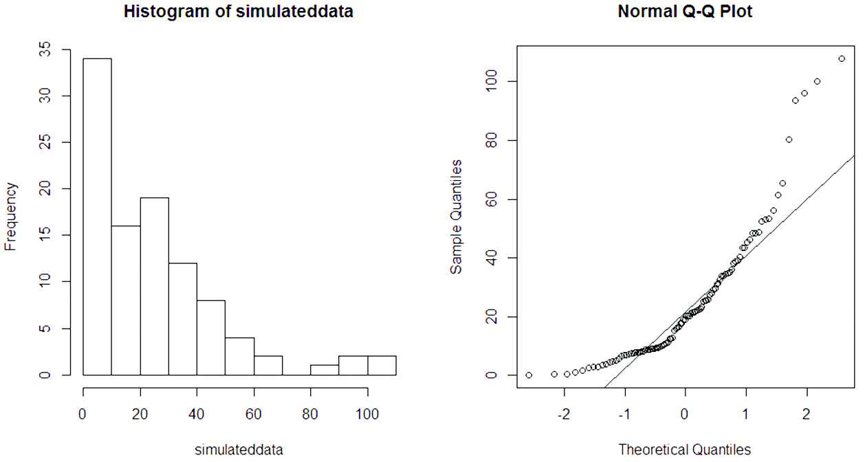
Histogram and normal Q-Q plot for simulated data show basic similarities with generalized asymmetric Laplace (GAL) distribution with respect to skewness, heavy tail and non-Gaussian.
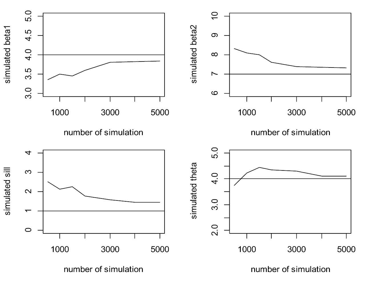
Plot of convergence for parameters.
Comparing the real and estimated values at these locations given in Table 1, shows plausible results. The used sample size
| Real Value | Real Value | ||||
|---|---|---|---|---|---|
| 30.54 | 30.50 (1.07) | 30.59 (1.13) | 183.33 | 183.34 (0.71) | 183.36 (1.40) |
| 14.40 | 14.25 (0.72) | 14.60 (0.96) | 34.11 | 33.99 (1.90) | 33.97 (1.81) |
| 15.30 | 15.34 (0.11) | 16.10 (0.74) | 16.14 | 16.30 (2.13) | 15.8 (2.30) |
| 57.81 | 57.80 (1.12) | 57.42 (1.06) | 17.52 | 17.91 (1.17) | 17.86 (0.90) |
| 65.02 | 64.98 (0.36) | 65.70 (0.60) | 34.08 | 33.92 (0.04) | 35.10 (0.11) |
| 19.60 | 19.54 (0.85) | 20.50 (0.76) | 9.47 | 9.63 (1.86) | 9.94 (1.64) |
| 4.41 | 4.23 (0.21) | 4.90(0.50) | 84.23 | 84.29 (2.09) | 84.72 (1.83) |
| 5.13 | 5.18 (1.00) | 5.63 (1.27) | 15.16 | 15.63 (0.14) | 15.87 (0.27) |
| 58.71 | 58.46 (.06) | 59.40 (0.49) | 66.74 | 66.71 (1.91) | 67.13 (2.13) |
| 3.71 | 3.77 (0.13) | 3.80 (0.09) | 64.98 | 65.42 (2.47) | 65.48 (2.58) |
Real values in 10 locations and their predictions (prediction error) for different models.
| Model | ||||
|---|---|---|---|---|
| Method | ||||
| PREMS |
0.374 | 0.560 | 0.547 | 0.810 |
The prediction mean of square errors (PREMS) in simulated generalized asymmetric Laplace (GAL) model for different models.
In order to have a knowledge about sensitivity of prediction with respect to the estimated parameters, we did predicted Z by assuming parameters,
5. APPLICATION TO REAL DATA
In this section, we analyze a real data set of 45 metals in 811 locations at a region near to Darab city of Iran. The histogram and Normal Q-Q plot of all metals show the skewness, heavy tail and non-Gaussian behavior of almost all data. However due to limited space we do not include all diagrams. The Histogram and Q-Q plot of two metals Sodium (Na) and Magnesium (Mg) have been shown in Figures 3. These two metals are selected because of their similarities to the GAL distribution. Figure 3, shows that GAL density functions has a good fitness to these data, where the parameters are estimated by using the maximum likelihood estimation method. Normal Q-Q plot of data shows that data are non-Gaussian. Also, the small p-values of Kolmogorov–Smirnov test and Shapiro–Wilk test for both two data set confirm that data are not Gaussian. In remainder of this section, we only consider Mg data. The scatter plots of data with respect to its coordinates given in Figure 4, show existence of some outliers in data, which we have ignored them for the time being. The scatter plots of 102 remained data show no trend in data.
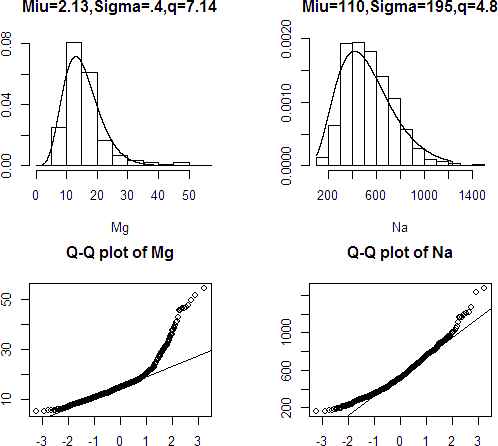
Histogram and normal Q-Q plot for metals Na and Mg.
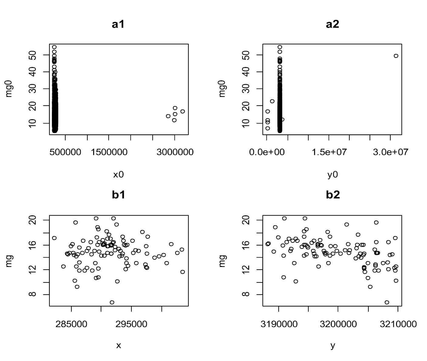
Panels a1 and a2 are scatter plots of Mg versus coordinates of locations and panels b1 and b2 are scatter plots of data with removed outliers.
We use 100 observations as the training set and 2 observations as the test set. Although we have used spatial covariance function throughout the paper, the variogram function is used for selecting a valid model. This comes from the fact that the variogram is more precise in model selection [19]. The empirical variogram of data is plotted in Figure 5.
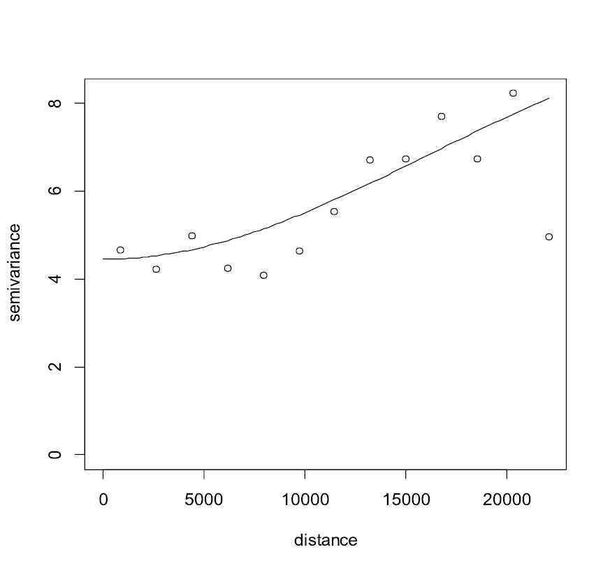
Empirical variogram and fitted isotropic exponential model.
The isotropic exponential model
| Predicted Value (Standard Deviation) |
||||
|---|---|---|---|---|
| Real Value | Kriging |
GAL |
||
| 15.29 | 15.52, NaN | 16.63 (1.86) | 15.29 (1.4) | 16.21 (3.4) |
| 18.05 | 19.45, NaN | 17.69 (1.87) | 17.93 (1.3) | 14.74 (2.8) |
NaN, refers to not a number.
Comparison between Kriging and generalized asymmetric Laplace (GAL).
This comparison shows the efficiency of GAL model with respect to Kriging. It is remarkable that using
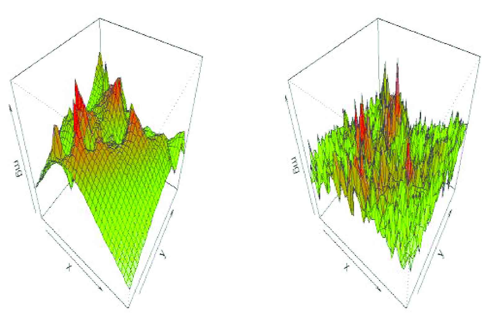
3D plot of surface prediction based on (left).
Contour graph of surface prediction is shown in Figure 7. Because of having an erratic shape of surface prediction based on
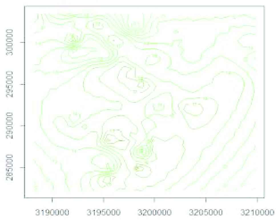
Contour plot of surface for predictions based on.
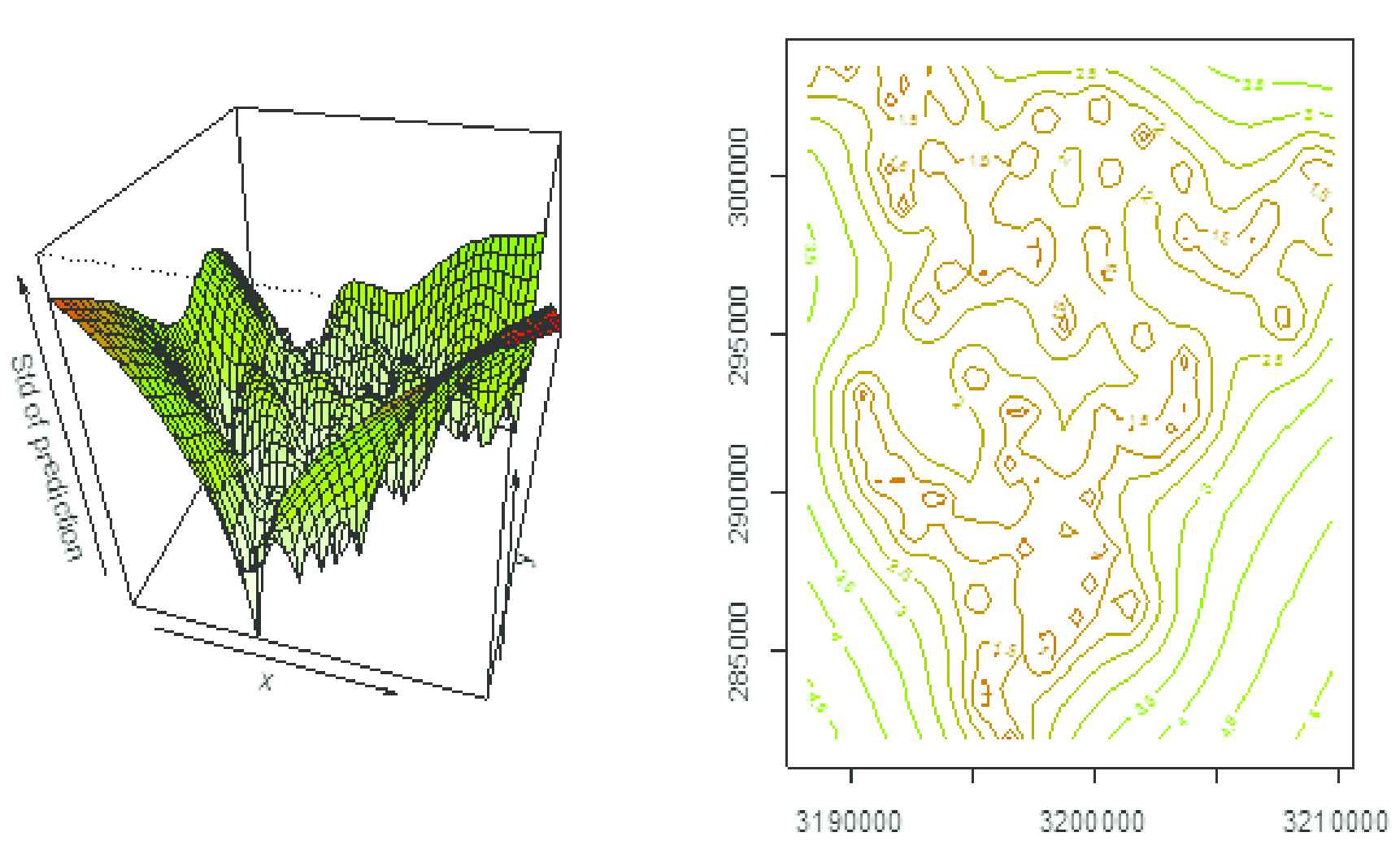
3D and contour plot of surface for prediction errors.
6. DISCUSSION AND CONCLUDING REMARKS
In order to define a RF in terms of the multivariate skew distributions, we propose the multivariate GAL distribution which is shown to be an appropriate choice for modeling skew and heavy tailed data. A Bayesian approach was then used for spatial interpolation. The simulation study and the analysis of a real data set show the reliable performance of this model. The proposed RF can be also used for many spatial purposes such as spatial regression and spatial generalized mixed linear models which have been previously studied by SN RF and CSN RF (see, e.g., Karimi and Mohammadzadeh [11] and Hosseini and Mohammadzadeh [13]).
CONFLICTS OF INTEREST
There is no conflicts of interest in this article.
AUTHORS' CONTRIBUTIONS
All authors have effective role in Sections 1–4 and 7. However, two other sections which is simulation and application and are concerned with programming in R, is only work of the first author.
Funding Statement
The work is sponsored by the Higher Education Center of Eghlid, Iran. None of authors have received Funding for this paper.
ACKNOWLEDGMENTS
The authors would like to sincerely thank the Editor-in-Chief and reviewers for their useful comments. The first author am also indebted to Higher Education Center of Eghlid for supporting this research.
REFERENCES
Cite this article
TY  - JOUR
AU  - Mohammad Mehdi Saber
AU  - Alireza Nematollahi
AU  - Mohsen Mohammadzadeh
PY  - 2021
DA  - 2021/01/20
TI  - Generalized Skew Laplace Random Fields: Bayesian Spatial Prediction for Skew and Heavy Tailed Data
JO  - Journal of Statistical Theory and Applications
SP  - 76
EP  - 85
VL  - 20
IS  - 1
SN  - 2214-1766
UR  - https://doi.org/10.2991/jsta.d.210111.001
DO  - 10.2991/jsta.d.210111.001
ID  - Saber2021
ER  -